Fuel is a vital resource in many engineering applications. This is especially the case of aerospace applications, where resources are strictly limited. Moreover, if resupplying is possible, it comes at the cost of very complex missions such as space rendezvous. From a control theory point of view, fuel consumption is often linked to actuator usage. Therefore, one of the main aspects emphasized when developing control algorithms intended for extra-terrestrial usage is minimizing resource consumption.
This post presents an HDL implementation of such a control algorithm, dubbed the “self-triggering Hands-off Control” algorithm, introduced in this article. Another relevant aspect involved in this implementation, is the method of solving linear programming optimization problems (LP), subject to both inequality and equality constraints. Finally, all the implemented procedures are optimized, from a hardware point of view, using various techniques such as buffer vectors, cached divisions and compilation directives (which will be discussed in the following sections).
Table of contents
- The Control Problem
- The Control Algorithm
- The Proposed Solver
- Vitis HLS & Workflow
- The Proposed Architecture
- Solving the KKT System
- Optimizing the hardware function
- Resource Consumption & Performance
- Conclusions
- Future Work
The Control Problem
Our attention is focused on a state-space model (this is a short intro in state-space representations) describing the translation dynamics of a satellite in orbit. The model is defined by the following equation:
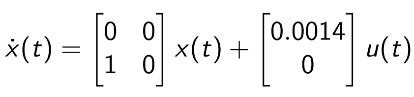
Here, the state is a vector consisting of the position and velocity of the satellite, measured on one axis, relative to a fixed point of the Earth’s orbit. The control signal, u(t), is the signal which commands the power exerted by a set of thrusters, capable of generating force in both directions. A positive u(t) would cause the satellite to accelerate in the positive direction of the axis, while a negative u(t) causes a deceleration. Naturally, as u(t) grows in magnitude the resources consumed by the thrusters, in order to produce force, will deplete faster. Therefore, minimizing the absolute value of u(t) is a critical measure in saving resources. The main goal is to drive the state of the system to the origin of the state space, i.e steer the satellite to the origin of the axis, and stop it there (maintain null speed and displacement).
The Control Algorithm
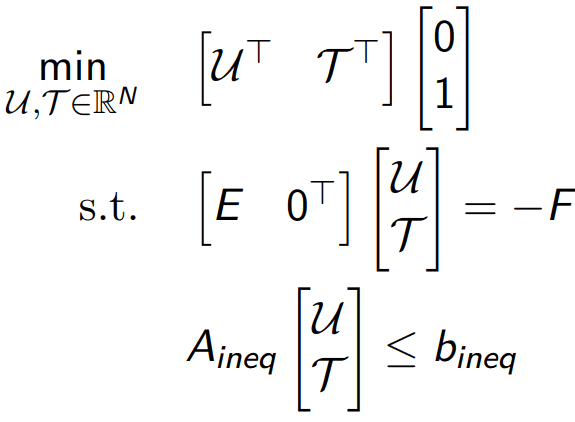
As presented in the previously mentioned article, this control algorithm aims to achieve the control objectives (which, in our case, will be to bring the satellite to the origin of the axis) while powering the thrusters for the shortest time possible (“keeping hands off the thrusters”). In order to do so, the authors have proposed a control scheme based on two optimal control problems: The Minimum Time problem and the L1 Control problem. For the first problem, based on the size and structure of the system, an analytical solution can be deduced, therefore not posing any problems from a computational point of view. The latter, however, will be treated as a numerical optimization problem, therefore consisting most of the effort which will be handled by the hardware platform. The resulting problem is:
Solving this problem results in a sequence of decisions regarding the propellers’ power, over a horizon of N sampling periods. As N grows, a prediction over a longer horizon needs to be done, resulting in a massive increase in complexity.
Before talking about the solver, chosen for the previously mentioned problem, another aspect needs to be discussed. The horizon length, N, varies from one iteration of the control algorithm to another (more details can be found in the article). The procedural approach of dealing with a varying horizon is to assign the exact required hardware resources each time the problem needs to be solved (allocating and freeing memory each iteration). In the world of hardware design languages (HDL), however, this is not fully possible.
For the final design, I chose to allocate the resources necessary for solving the L1 Control problem over a maximum horizon of length Nmax (equal to 300). The actual size of the problem to be solved at each iteration is then indicated by the size to which a matrix is filled with elements. By leaving the rest of it empty, only the necessary control signals will be provided in the final solution.
The Proposed Solver
After a thorough analysis of multiple solvers, designated for LP problems, I have come to the conclusion that ADMM (Alternating Direction Method of Multipliers) is the most suitable choice, taking into consideration the constraints to which the problem is subject to. The manner of treating both types of constraints, without the explicit need of projecting on any space other than multi-dimensional box-type intervals is what makes this solver appealing to both the problem and the chosen hardware platform. Moreover, each iteration of this solver solely relies on solving a linear system of equations, a task which can be easily handled and parallelized in the HDL realm. The system to be solved, also called the KKT (Karush Kuhn Tucker) System, is of the following form:
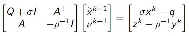
The matrix on the left hand side of the system is only composed out of the elements defining the optimization problem, thus it is constant throughout the entire functioning time of the ADMM algorithm. This will be further exploited to reduce the computation time and, consequently, the response time of the control algorithm.
Vitis HLS & Workflow
As FPGAs are widely considered to be a very popular choice for accelerating execution time of computationally complex tasks, I wanted to explore their capabilities in the realm of control engineering. The continuous possibility of trading fine performance for resource consumption creates an appropriate environment for developing optimized hardware implementations of pre-tested software algorithms, whilst obeying constraints concerning design area, response time and output precision.
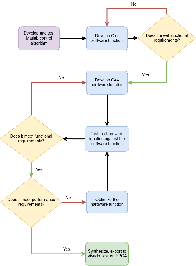
The main drawback in FPGA development, however, is the reduced speed at which solutions can be implemented using HDL. Nonetheless, as industry started to show more interest in the potential of this type of hardware platform, a solution to the previously mentioned problem emerged, namely High-level Synthesis tools (HLS tools). This type of software allows for a high-level language code (C++, Python, OpenCL, MATLAB, SystemC) to be converted to HDL modules, therefore shortening the overall development time. However, aside from developing the algorithm using the high-level language, the developer will also have to focus his attention on the resulting module’s performance and update the “top level” function accordingly, with the scope of achieving a desired behavior. The workflow of this project is illustrated in the following figure:
The Proposed Architecture
Taking into consideration the two problems that need to be solved, I have proposed the following hardware architecture. The two sub-modules (Minimum Time and L1 Control) handle the two control problems, while input and output communication is done with the help of AXIS interfaces. This protocol allows the transmission of large amounts of data in high-rate bursts, which is essential for transferring vectors or matrices.
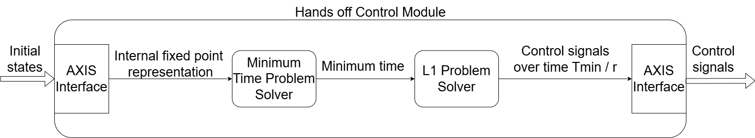
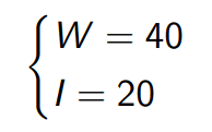
Regarding the internal representation of the algorithm, I have opted for a fixed-point representation, as operations can be directly executed using the logic elements of the board, without any need of emulations, as in the case of floating-point operations. This also allows for a custom word length to be chosen, therefore allowing for the memory consumption to be adjusted as required. Nevertheless, the main disadvantage in using this type of representation is the limited precision it offers. As there are plenty of multiplications, divisions and other operations that require a finer representation, or that can lead to an overflow, a fixed-point representation of the following dimension was chosen:
Solving the KKT System
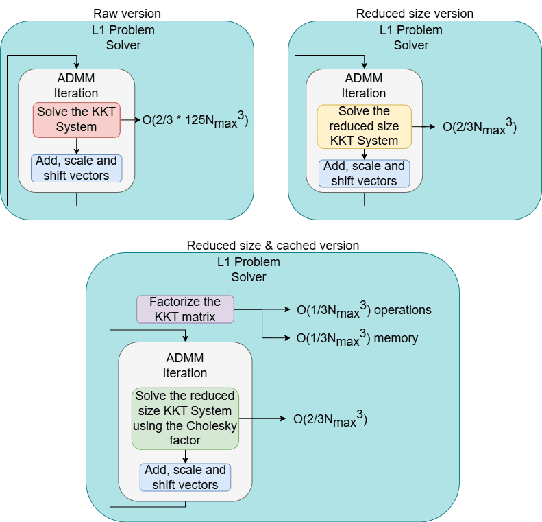
As the Minimum Time problem has been solved analytically, the main challenge in designing the hardware module lies in developing an efficient method of solving the KKT System of equations. For this matter, two remarks have allowed for a massive improvement in the throughput of the module.
Reducing the system size
The first step I took in reducing the computational effort of the ADMM iteration is to reduce the size of the KKT system of equations. This can be done by using the block forms of matrices A and Q and by appropriately partitioning the variables composing the unknowns of the system. Henceforth, from an initial dimension of 5 * Nmax + 2, the resulting reduced size is Nmax.
To emphasize the improvement, suppose a classical Gaussian elimination algorithm was used as a solver. The size reduction would lead to a drop in complexity from O(2/3*(5Nmax+2)3) to O(2/3*Nmax3), which is, indeed, a significant improvement.
Caching the matrix
To further enhance the response time of the algorithm, another optimization can be done, by exploiting another interesting property of the KKT system. Recalling equation 3, we noticed that the matrix of the system is constant throughout the entire execution time of the algorithm. Moreover, it is a positive semidefinite matrix, thus admitting a special type of factorization called Cholesky factorization. This factorization is obtained at the cost of O(Nmax3/3) operations. Following such a factorization, done before the initialization of the algorithm, the equation system can be solved using a particular method, involved for solving triangular systems. This way, the complexity drops again, from the previously invoked O(2/3*Nmax3), to a new O(Nmax2). However, this comes at the cost of storing the Cholesky factor, taking up a block of memory of size 0.5*Nmax2.
The evolution of the ADMM iteration, along with the overall L1 problem solver, with respect to all the improvements done, can be observed in the following picture:
Optimizing the Hardware function
In addition to the previously discussed improvements, which significantly decreased the complexity for each iteration, Vitis offers a set of directives called “pragmas” which allows the designer to reshape the resource assignment in a more favorable manner.
Nested loops
In order to reduce the complexity of nested loops, pipelining can be applied. Applying a pipeline pragma to an outer loop would lead to its contained loops to be unrolled (parallelized), leading to a massive increase in resource consumption, traded for a noteworthy decrease in execution time. For this hardware implementation, I chose to pipeline the inner loops, thus shortening the execution time of one iteration of the outer loops, without excessively consuming hardware resources. However, for the pipeline to be successfully applied, the loop must either have a fixed number of iterations, or a known trip count (minimum number of iterations).
To achieve this condition, nested loops structures have been modified according to the following scheme:
Initial Nested Loops Structure
for(i = 0; i < n; i++) {
    /* Outer loop instructions involving a variable n_temp*/
    for(j = 0; j < n_temp; j++) {
        /*Inner loop body*/
    }
}
Modified Nested Loops Structure
for(i = 0; i < n; i++) {
    /* Outer loop instructions involving a variable n_temp*/
    for(j = 0; j < n; j++) {
        if(j <= n_temp) {
            /*Inner loop body*/
        }
    }
}
Accessing the Cholesky Factor
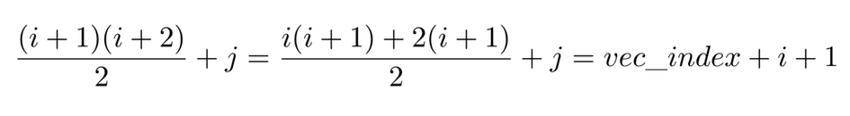
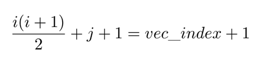
It was mentioned earlier that, after factoring the KKT matrix, the system of equations can be solved using a triangular solver routine. This is due to the Cholesky factor being a triangular matrix (lower or upper, depending on the implementation). Therefore, if stored as a two dimensional array, it would only occupy half of the assigned space. As a measure of saving memory, I have opted for storing the factor in a one dimensional array. This saves up some space, but leads to a more complex manner of accessing elements of the factor:
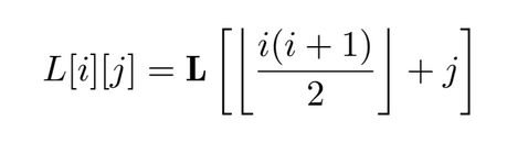
Accessing one element now requires two additions, multiplication and a division (or bit shifting). This sequence of operations cannot be executed in less than a clock cycle at an imposed clock frequency of 100MHz. This raises problems when trying to pipeline the loops included in the Cholesky factorization routine, as the contents of a loop including the Cholesky factor cannot be executed in one clock cycle. To overcome this issue, whenever iterating through this factor row-wise or column-wise, the starting index is pre-calculated and further incremented according to one of the following two rules:
Resource Consumption & Performance
| BRAM_18K | DSP | FF | LUT | |
| Total | 262 | 213 | 25955 | 47474 |
| Available | 280 | 220 | 106400 | 53200 |
| Utilization(%) | 93 | 96 | 24 | 89 |
The total amount of resources figured in the table is of a PYNQ-Z1 development kit, used as a reference hardware platform. As it can be seen, memory and DSP and LUT consumption are very close to the maximum cap, while the Flip-Flop consumption is comparatively low. The memory consumption is mostly caused by the Cholesky factor, while the DSP consumption results from the multiple divisions that have to be done in order to compute this factor.
The response time of the algorithm is of 1.43 * 109 clock cycles. For a clock period of 10ns, this is equivalent to 1.43 seconds. In the context of this control problem, the proposed sampling period is of 6.28 seconds, which means that the response time of the control algorithm complies to any timing constraints.
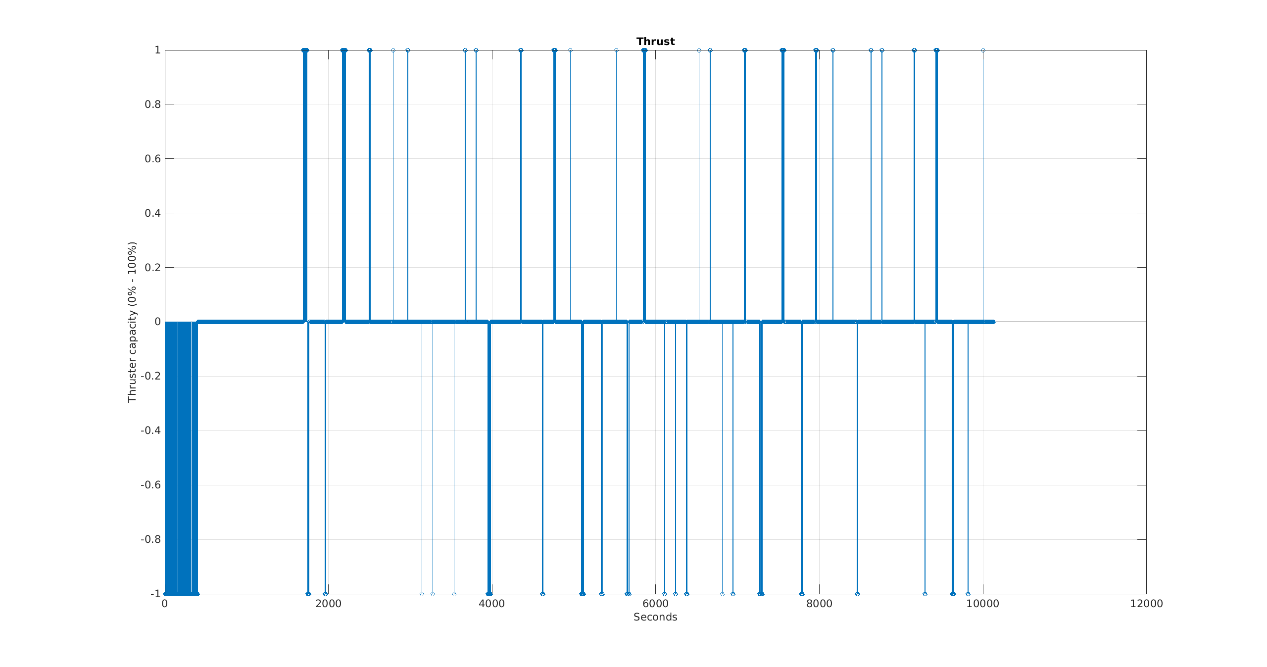
In order to check the functionality of the control algorithm, a simulation has been done. Throughout the simulation, the control algorithm provides the thruster command signals, followed by the simulation of the thrusting effect on the satellite. Additional to this, a stochastic disturbance is involved. Its purpose is to model orbital effects that may interfere with the natural trajectory of the body (gravitational anomalies, atmospheric drag, sun pressure).
The following plot illustrates the control signals generated by the hardware algorithm, over time. This was obtained through a simulation done in Vitis. It is worth noticing that for most of the time, the control thrusters are turned off (set to 0%). More exactly, the on-time is only 12.83% of the total simulation time, of approximately 3 hours of simulation.
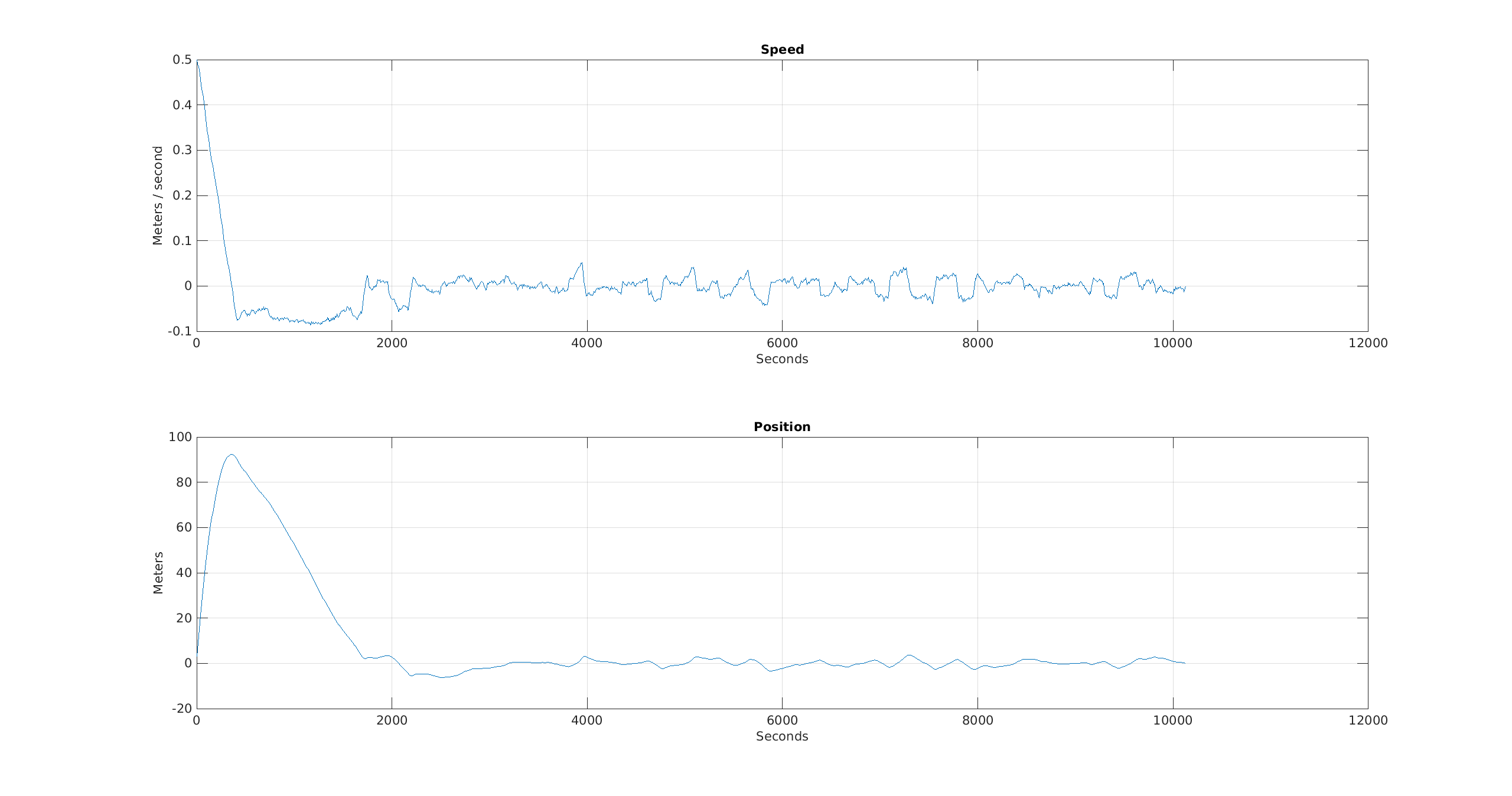
The resulting position and speed evolution of the satellite is figured below. The initial position of the satellite is 3 meters away from the desired position. Moreover, it is moving in the same direction (as the displacement) with a velocity of 0.5 m/s. This causes a large overshoot in the position of the satellite, after which the control algorithm steers it to the target position, keeping it there for the rest of the simulation. The effect of the disturbances can still be seen in the speed evolution over time. Nonetheless, these disturbances do not have a significant effect on the position of the satellite, as the control algorithm brings corrections whenever needed.
The MATLAB double precision floating-point algorithm response time is approximately 0.71 seconds, for a 10-core Intel I7 Processor. This is half of the response time of the hardware module. This difference in speed can be pointed towards the high memory requirements of the solution itself. Usually, the L1 control problem would require storing multiple matrices, which are further used in finding the solution. In order to avoid memory overflows, I have opted for an on-the-spot computation of some of those matrices. This saves up memory, at the cost of an increased number of operations.
The way the Cholesky factor is stored also impacts the performance of the algorithm. Multiple I/O operations at once are only possible if the memory storing the variable is partitioned according to some pattern. This pattern implies dividing the array in multiple segments of equal lengths. The elements of the Cholesky factor, however, form a triangular matrix, thus cannot be logically distributed in equal-sized containers.
Conclusions
After a thorough analysis of this subject, I have come to the following conclusions:
- Trying to work only with the internal memory of the FPGA is not the best approach. An external memory would free up the internal space and allow for more area optimization of the algorithm itself.
- The output of the hardware module is highly dependent on the precision of the fixed-point representation. This led to the choice of the current fixed-point representation size. A more precise representation would lead to less errors, but would also cause an increase in the area of the module.
- The hardware implementation of the control algorithm achieves its purpose of steering the satellite to the desired position, even under the presence of external disturbances.
Future work
Future improvements that can be brought to the hardware implementation are mainly related to the manner in which the L1 control problem is solved. For larger systems (more states / coordinates), an external memory should be involved, as there won’t be enough internal space on the hardware platform to store all the necessary arrays. For particular systems, such as the system involved in this problem, an analytical way of solving the L1 control problem can be researched. This would reduce all the iterative procedures to a few computations.
Steps to reproduce
The project source code, along with the MATLAB reference model can be downloaded from AMIQ’s GitHub Repository.
- Create a Vitis HLS project
- Add all source & testbench files
- Synthesize & Simulate the hardware module
- A trajectory analysis can be done by copying the contents of “state_file.dat” and “hardware_output.dat” in the MATLAB folder and running “parse_plot.m” script
Software used for creating this project:
- OS: Ubuntu 22.04.2
- Vitis version: Vitis HLS 2023.2
- MATLAB version: MATLAB R2023b