All scripts, architectures, implementation details and usage examples discussed in this article are available in the project GitHub repository: amiq_plcust.
Introduction
Debugging is a consistent part of the verification engineer’s time, whether we talk about RTL bugs or testbench bugs. In fact, according to the 2022 Wilson Research Group Functional Verification Study, almost half of the verification engineer’s time is spent debugging (as is depicted in Figure 1). That’s what sparked the idea of this project, which aims to provide novel insights into the large database generated by a regression, accelerating the tedious task of debugging.
In the context of developing a verification environment, functional bugs can be of various “shapes”, because parts interacting on multiple integration levels are involved, such as verification components, blocks, systems, or even development visions. Some defects pertain to the logical code of the design, while others can relate to the verification environment: internal errors, erroneous connections, or stimuli that do not conform to protocol specifications. Additionally, the defects strongly depend on the development stage of the verification project, and the key to resolving them lies in good communication between the designer and the verification engineer.
Regardless of the bug cause, debugging in the context of functional verification is a laborious and lengthy process. The cumulative experience of verification engineers has led to a traditional debugging method, which involves investigating the error message encountered earliest in a simulation. This ensures isolation of the bug, guarantees that it is not triggered by a possible prior problem, and solving it could determine and eliminate subsequent errors in cascade. However, the effort to determine the cause of the bug remains an intellectual one, of the verification engineer. The difficulty lies in the fact that the bug with the shortest chain of logical events is hard to identify, and investigating error messages consumes most of the time. Ideally, the most frequently encountered and widespread bug should be resolved with priority.

Figure 1. Where ASIC verification engineers spend their time.
Table of Contents
- Problem
- Solution
- Requirements overview
- Workflow
- Proposed clustering methodology
- Use Case Evaluation & Comparison
- Conclusions
- References and resources
- Acknowledgements
1. Problem
When a bug-infested RTL is analyzed using a properly set-up testbench, checks/assertions act as tripwires, intended to catch any behavior that does not comply with the design specification, and which may also be manifestations of a design bug. A failed assertion throws an error message, and it is the duty of the verification engineer to map these failure messages to the bug root-cause. However, the way multiple bugs interact and correlate to the assertions set up in the verification environment is where things become weird. Just like in healthcare, the symptoms that are detected through medical checks need to be reviewed to determine the root cause (aka disease) that is affecting a patient. Error messages are just symptoms of a bug, but putting error messages together cleverly can help an engineer track down the causes of a bug and fix design flaws.
Current EDA tools only provide ways to group together runs in a regression using the error message as a grouping criteria. This method implies that there is a 1:1 correlation between an error message and the bug attempted to be identified. This is not always the case, as one bug can manifest through multiple error messages (1:N), and the same error message can be linked with multiple bugs (N:1). These relations are depicted in figure 2. What would be handy is a smart way to cluster together runs based on the failure root-cause, and not on the error message.
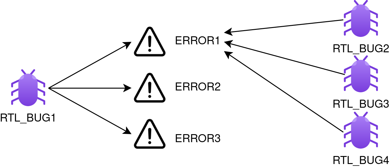
Figure 2. Bug to error message mapping.
2. Solution
To outline a methodology for grouping together functional verification runs based on the cause of failure, the error messages are not enough. Every run needs to be defined as a separate collection of verification intentions, controlled by flags from the highest level of abstraction, in order to turn a regression into a valuable database. In fact, what separates test cases between each other in CRMDV (Constraint Random Metric-Driven Verification) fashion, is the way the stimuli sent to the RTL are being constrained. This means that a distinct functional verification test case, where verification functionality is controlled by high-level abstract flags, represents the result of the interaction between these verification intentions. The ability to define a scenario through abstract verification parameters is enabled by the Externally Controlled Test Bench (ECTB) framework, using plusargs files. The goal is to apply suitable clustering algorithms on the database of parameters and error messages, in order to discover inherent structures and uncover hidden insights about the causes of the failures.
For instance, the case study used for the initial development of the project was a block that computes the determinant of a 3×3 matrix. The block works in a simple manner: the elements of the matrix are sent in order from top-left to bottom-right, mat_request is a backpressure signal, and after the input transaction the result is immediately driven out (marked with overflow if it is the case). The interfaces of the Matrix Determinant block can be noticed in Figure 3.
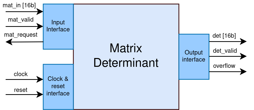
Figure 3. Project case study: the Matrix Determinant block.
The way one would implement a constrained scenario to send long bursts of permutation matrices only, with one initial reset, would translate in ECTB to the plusargs file in Figure 4. All of the abstract parameter values have to be implemented by the user into SystemVerilog constraints, as required by the framework. In this particular case, amiq_md_base_seq is a sequence that extends amiq_ectb_sequence and that implements the constraints mapped to the values retrieved through the register_all_vars() function.
+seq0=amiq_md_base_seq
+seq0_name=general_sequence
+general_sequence_nof_items=large
+general_sequence_nof_resets=initial
+general_sequence_delay_type=small
+general_sequence_matrix_type=permutation
Figure 4. Example of ECTB testcase implementation using plusargs.
3. Requirements Overview
From a high-level view, the most basic requirements of the explored solution are:
- Design the stimuli constraints such that the user can have a centralized external control layer (implemented in the project through points 1 and 2 below).
- In the VE, Include implementation methods that enable facile stimuli constraint extraction and labeling (enabled in the project through point 3 below).
- Use languages and methodologies that allow for post-simulation big data processing (deployed in the project through point 4 below).
In our case, these requirements were implemented as follows:
- Development of the verification environment using ECTB architecture and principles.
- Implementing a high-level of abstraction, enabling the verification environment to be governed by a single general sequence. This employs abstract control parameters, with discrete values (parameters with a wide range of values, such as 32-bit integers, may not lead to concrete results and do not offer a clear debugging direction).
- Transparency of values used for all control parameters of a test scenario, by displaying these in the associated run log, regardless of whether they were defined in the plusargs file.
- Dependencies on the following non-standard Python packages: NumPy version 1.21.5, pandas version 1.3.5, Plotly version 5.18.0, Dash version 2.16.1, scikit-learn version 1.3.2. All of these are documented in the README.txt file of the project repo.
4. Workflow
The project employs 3 execution phases (outlined in Figure 5), which take place right after a regression has finished:
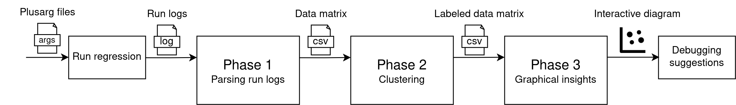
Figure 5. Project execution phases.
1. Constraints parameter extraction: This stage involves parsing the information from the regression’s run logs, aiming to construct a database of abstract parameters and error messages, as indicated in Figure 6.
| Run \ Feature | Parameter1 | … | Parameterj | … | ParameterN | Status |
| run1 | value11 | … | value1j | … | value1N | error1 |
| … | … | … | … | … | … | … |
| runi | valuei1 | … | valueij | … | valueiN | errork |
| … | … | … | … | … | … | … |
| runM | valueM1 | … | valueMj | … | valueMN | errorK |
Figure 6. Generalized regression database
Because in ECTB parameters can be registered with a default value without requiring a +plusarg, a change was added to the existing variable register functions in ECTB to display all values in the run log using the format “+var_name=value”. This is added in the ECTB submodule available with the amiq_pclust repo.
| run_name | nof_items | nof_resets | delay_type | interesting_matrix | delay_pattern | exact_value | error_type |
| run_1 | small | initial | medium | no | N/A | N/A | error1 |
| run_2 | large | initial | b2b | no | N/A | N/A | error3 |
| run_3 | medium | small | medium | no | N/A | N/A | error3 |
| run_4 | small | initial | N/A | N/A | 5-10 | one | error1 |
| run_5 | small | initial | N/A | N/A | 10-15 | almost_ovf | error4 |
| run_6 | small | initial | medium | no | N/A | N/A | error1 |
| run_7 | large | initial | b2b | no | N/A | N/A | error4 |
| run_8 | medium | small | medium | no | N/A | N/A | error1 |
| run_9 | small | initial | N/A | N/A | 5-10 | one | error2 |
| run_10 | small | initial | N/A | N/A | 10-15 | almost_ovf | error2 |
Figure 7. Example of a Matrix Determinant regression database
The N/A value associated with some parameters in Figure 7 is not an error and is in itself an interesting topic. Although a general abstract high-level sequence is required for the project, that does not mean that the same sequence type has to be used across all testcases in a regression. Different sequence types can be used, which utilize different verification parameters, meaning that some parameters may be encountered in multiple sequences, while others can be specific flags used for directed targeting of functionality. The purpose of the project was to offer debugging insights global to a regression, meaning that different verification parameters used across multiple sequence types and tests should be accumulated in the same database. Whenever a parameter is encountered with the N/A value for a run, it means that the sequence type used for that run does not utilize the parameter, and this value does not contribute to the clustering process.
2. Clustering: Running a clustering algorithm, specifically either DBSCAN, HDBSCAN, or OPTICS, on the database constructed in the first stage. The objective is to obtain labels for each run in the regression, with each group of runs providing traces of a bug.
Because the number of bugs encountered in a regression is unknown, and “bug traces” clusters do not respect a statistical distribution, the project adopts a clustering model using density-based algorithms. The similarity between the features of two runs indicates a spatial proximity between them, accommodating metrics calculated in non-Euclidean spaces. Algorithms as such can capture the relationship between runs in an ECTB regression, with built-in support for directed tests (noise). In this context, a noise point is a run that uses parameters completely different from the majority of the regression runs, standing out as atypical.
The clustering approach is rather unconventional, because the space of individuals is not a numerical one, but an abstract space of verification parameters. Initially, we actually tried mapping numerical values to each distinct verification parameter value, but this idea was later dropped as it did not represent a suitable method of clustering categorical data. Attributing a numerical value to a verification parameter is like trying to place abstract concepts on an orderable numerical axis, which in most cases is not an accurate model, but still one with great impact on the results of the clustering process. Another proposal was to group parameters that are semantically linked (such as delay_type and delay_pattern, for the Matrix Determinant case study), and assign them closer numerical values or place them on correlated axes. But again, this grouping is a subjective problem in itself and would make the project dependent on the testbench implementation.
3. Graphical insights: This step involves transforming the labeled database into an n-dimensional interpreted Sankey diagram using the Plotly Python library, and which is depicted in Figure 8. In this chart:
- columns represent features;
- nodes are the discrete values of a feature;
- a connection between nodes represents an interaction between the parameters (co-occurrence in a run);
- colors of the connections signify the trace of a bug;
To further simplify visualization and offer the user more flexibility, a series of filters are implemented in a Dash GUI. Following the execution of the proposed script, an interactive application is obtained that provides a general perspective on the relationships between all verification parameters used in a regression. Finally, the suggested debugging direction is presented in the form of a table (as shown in Figure 9), which includes the most frequently encountered combinations of parameter values that have caused errors.
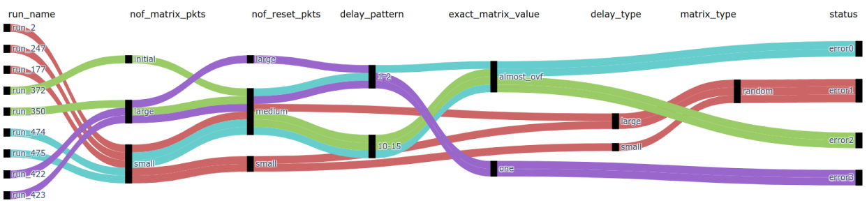
Figure 8. Interpreted Sankey diagram of a regression.

Figure 9. Debugging suggestions table.
4.1. User Mode
After cloning the amiq_pclust GitHub repository, it is required to install all Python libraries as specified in the README.txt file. The script that encapsulates all three stages described earlier is “amiq_pclust/amiq23_md/scripts/regression_analysis.py”. When users intend to run a regression on an ECTB testbench, in order to subsequently visualize the interactive diagram and debugging indicators, they should include the regression_analysis.py script in the regression definition file (Verification Regression Specification File, VRSF) as a post-session script, which includes the path to the regression directory. This working flow is represented in Figure 10.
The script can also be run manually by specifying the path to the regression directory:
$ python3 regression_analysis.py –path <path/to/reg_dir> [-u] (includes passed runs) [-g] (generates regression database in csv format)
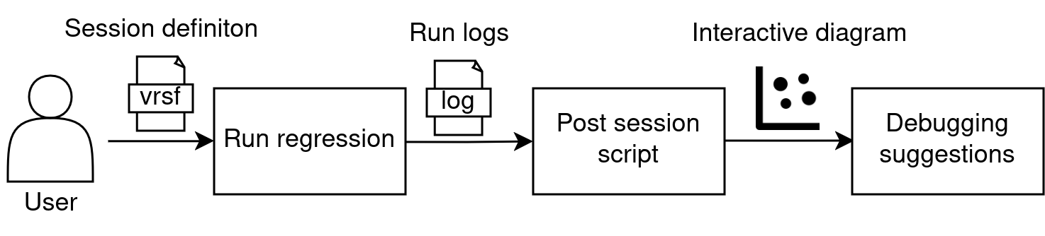
Figure 10. User interaction flow.
4.2. Developer Mode
The next goal of the project was to identify a clustering methodology that would be suitable regardless of the target testbench. DBSCAN uses the hyperparameters eps (an evaluation radius for areas of interest) and minPts (nof_infividuals threshold that dictates what areas are of interest), while HDBSCAN and OPTICS only require setting minPts. A simple, but deceptive step to take in this project was to optimize the methodology in a Matrix Determinant-biased manner. To avoid introducing block dependencies into the clustering methodology, a variety of case studies was required, but the IPs available were limited and converting multiple testbenches to ECTB would have been time inefficient for the project. This is why a method to inject synthetic bugs into a sandbox environment and measure the clustering performance was needed, virtually modeling any RTL and any bugs, which we called the “Developer Mode” of the project.
The following scripts and files presented are located at “amiq_pclust/amiq23_md/scripts/development”. The script that generates the synthetic bugs and injects them in the testbench is bugs_generator.py. These synthetic bugs are implemented as SVAs (SystemVerilog Assertions) in the testbench and can manifest through different error messages (even different bugs with the same message), but they are uniquely associated with a specific combination of ECTB parameters. The parameter values and names are abstracted in the format “param_X” (where X is an uppercase letter from the English alphabet) and “val_Y” (where Y is a positive integer), and the error generation conditions are configurable by the developer controlling the sandbox environment through the bugs_generator_config Excel file. The synthetic bug to error message mapping is depicted in Figure 11. In this case, N/A means that the sequence type through which the bug can be detected does not utilize the corresponding parameter, while any means that the parameter is used by the sequence type, but is not associated with the bug (meaning it can take any value without influencing).
| bug | error | nof_items | nof_resets | delay_type | matrix_type | delay_pattern | exact_value | seq |
| bug_3 | error2 | small | medium | any | permutation | N/A | N/A | seq_0 |
| bug_2 | error0 | initial | any | N/A | N/A | 10-15 | any | seq_1 |
| bug_1 | error1 | any | large | small | random | N/A | N/A | seq_0 |
| bug_0 | error1 | any | large | any | random | N/A | N/A | seq_0 |
Figure 11. Example of synthetic bugs generation for the Matrix Determinant case study
Once a set of bugs is randomly generated (as a combination of parameter values), the bug-parameters association is encoded in binary format (codes which are subsequently transposed into SVA files included in the testbench). Additionally, a configurable number of plusarg files (corresponding to a test) can be generated for each sequence available in the sandbox environment, alongside a VRSF that encompasses them into a regression. Running the three basic stages of the proposed project allows comparing the conclusions of the debugging suggestions table with the signatures of the initially generated bugs (reference model). For a practical example consult the Developer Mode User Guide. The structure of the sandbox environment is described in Figure 12. Overall, the purpose of the sandbox environment is to qualify the clustering stage for any kind of testbench.
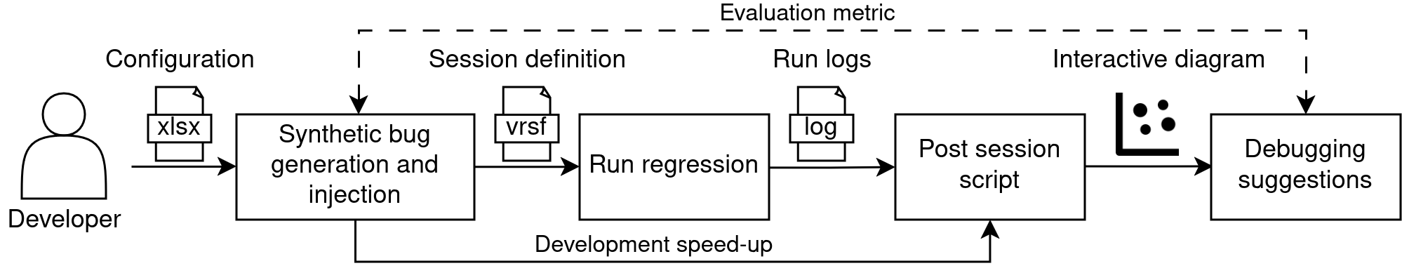
Figure 12. Developer interaction flow.
Differences from the User Mode:
- The plusargs files and VRSF can be produced by the generation and injection block.
- Based on the generated labels and those captured by the clustering algorithm, an evaluation metric of the grouping can be calculated, which in the case of this project is the F1 score (described later). This score is displayed interactively in the application’s GUI, alongside the percentage of noise (the sandbox GUI is launched using the clustering_visualize_sandbox.py script).
- In the generation and injection block, all the parameter information for the tests to be generated is already present, alongside the faulty parameter combinations and their associated error messages (from the model based on which SVA files are generated). Thus, to overcome regression runtime, from the generation and injection block one can directly obtain the regression database and speed-up development.
4.3. Interactive GUI
Depending on the testbench complexity and regression size, a Sankey diagram can be difficult to interpret. This is why the Dash GUI of the project showcases multiple features to filter tests and focus on corner-cases, working interactively through a system of customized callbacks. These features, which are accessed through the text fields shown in Figure 13, are:
- Reorder parameter column order;
Usage: param_A, param_B, param_C, …
! Important Note: omitted parameters are excluded from the diagram.
- Single out run;
Usage: run_1, run_2, run_3, …
- Single out cluster;
Usage: bug_1, bug_2, bug_3, …
- Single out parameter value;
Usage: param_A$val_0
- Color customization;
Usage: Choose cluster and available color from dropdown lists.
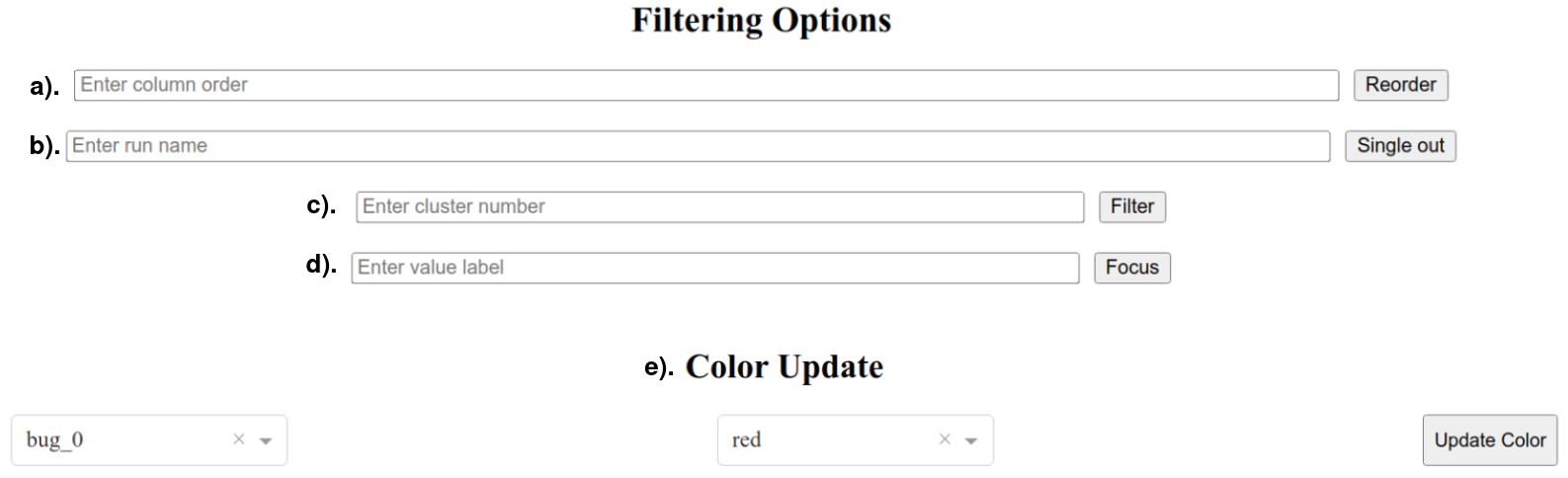
Figure 13. Dash GUI filtering options.
Besides these, the application most importantly features dynamic clustering, meaning that the user can interactively change the clustering algorithm or hyperparameter values, and the diagram will change on-the-go, as shown in Figure 14.
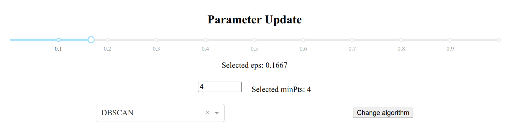
Figure 14. Dynamic clustering control knobs.
5. Proposed clustering methodology
Based on the indications provided by the creators of DBSCAN in “DBSCAN Revisited: Why and How You Should (Still) Use DBSCAN” , and after several iterations of trial and error, the proposed clustering methodology is described in the following subchapters. Note that this methodology is used as the default for clustering ECTB regression runs, but the user has complete control over what hyperparameters are used for each algorithm if he considers they better suit the context of his testbench.
5.1. Distance
As foreshadowed in Chapter 4, the space in which the clustering algorithm is applied is non-Euclidean, where the distance calculated between individuals is the Dice-Sørensen distance (DDS) and is calculated as DDS = 1 – CDS, where CDS ∈ [0,1] is the Dice-Sørensen similarity coefficient:
CDS = 1 → DDS = 0 → Identical individuals
CDS = 0 → DDS = 1 → Completely different individuals
To calculate the Dice-Sørensen similarity coefficient between two runs, each run ( individual, point) should be viewed as a set. If two verification parameters use the same name for values (in the case of Matrix Determinant, nof_matrix_pkts and nof_reset_pkts can both have small and large values), then these will be treated individually (e.g. nof_matrix_pkts_small and nof_reset_pkts_small). Thus, CDS between two sets A and B is:
CDS = 2|A∩B| / (|A|+|B|)
meaning twice the number of common elements of the two sets, divided by the sum of the cardinalities of the two sets. As motivated in Chapter 4, the N/A values are ignored. The distances between individuals are represented in a symmetric matrix with respect to the main diagonal, of dimension MxM, where M is the number of regression tests (depicted in Figure 15). The element of the distance matrix located on row i and column j represents the Dice-Sørensen distance between test i and test j (i == j => DDS = 0).
| Run \ Run | run1 | … | runj | … | runM |
| run1 | DDS11 | … | DDS1j | … | DDS1M |
| … | … | … | … | … | … |
| runi | DDSi1 | … | DDSij | … | DDSiM |
| … | … | … | … | … | … |
| runM | DDSM1 | … | DDSMj | … | DDSMM |
Figure 15. Dice-Sørensen distance matrix of ECTB regression database.
5.2. Epsilon
The hyperparameter ε is determined using the K-nearest neighbors (KNN) algorithm, based on each run from the Dice-Sørensen distance matrix. The value of K was determined heuristically, being the integer part of √(number of failed tests). The algorithm for determining the optimal value of ε is presented in the following section:
1: Distance list ← the KNN for each run.
2: Coordinate list x ← integer interval [0, M]
3: Coordinate list y ← distance list sorted in ascending order
4: Create a scatter plot of x and y coordinates (KNN graph, as in Figure 16) ▷ This shows the separation between points close to the rest of the set, and noisy points
5: For each x, y pair determine curvature κ ← |x′′y′−y′′x′|/((x′2+y′2)3/2)
6: εoptimum ← index of first 0 value in curvature list ▷ First plateau in KNN graph
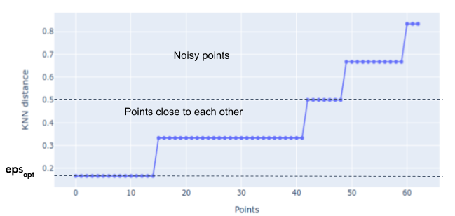
Figure 16. Determining the optimum eps on KNN graph.
5.3. MinPts
The hyperparameter minPts is the only one to be optimized for the HDBSCAN and OPTICS algorithms, while in the case of the DBSCAN algorithm, it is optimized alongside ε. According to the heuristic method presented in the paper “ST-DBSCAN: An algorithm for clustering spatial–temporal data“, the hyperparameter minPts is set as the integer part of the result of ln(number of failed tests), where minPts ≥ 2. The advantage of this method is that the hyperparameter minPts scales with the size of the dataset. In datasets with a high number of points, the density zones evaluation criterion will be stricter, while in datasets with a lower number of points, the criterion will be more permissive. This aspect aligns the density-based grouping model with the regression model, whose number of tests varies depending on the verification engineer’s intentions.
5.4. Metrics
Within the sandbox environment, an evaluation metric for the clustering process can be calculated. The chosen evaluation metric is the F1 score ∈ [0, 1], which represents the harmonic mean between precision and recall measures (the F1 score will have maximum value when precision and recall values are equal). These are calculated through an adapted method, where the generated clusters and the ideal ones are compared individually. It is important to specify that clusters are not compared by labels but by the best overlap (clusters that have the most points in common). When evaluating precision and recall individually between clusters, the values used in calculating the F1 score will be the arithmetic means of these values.
precisioni = TP/(TP + FP)
recalli = TP/(TP + FN), where i ∈ [0, number of clusters]
F1 score = (2 * precisionmean * recallmean)/(precisionmean + recallmean)
- TP represents the number of points correctly identified by the clustering algorithm (true positives);
- FP are points that are incorrectly identified (false positives);
- FN are points that are not identified by the algorithm, although they should appear in the corresponding group (false negatives);
Thus, precision measures how many of the grouped points are correct, while recall measures how many of the reference model points are identified. The closer the F1 score is to 1, the better the clustering results reflect the reference model. Additionally, as the percentage of noise points increases, the F1 score will be lower (noise is considered as FP). This evaluation metric takes into account both that the identified points are correctly grouped, and that the resulting model includes as many points as possible from the reference model.
6. Use Case Evaluation & Comparison
A comparative analysis was conducted of the three clustering algorithms studied in this project, across three distinct case studies, regarding the F1 score. These cases represent three specific situations of bug generation using the sandbox environment. Each case is evaluated for three regression sizes (100, 500, and 1000 runs), and compared against the three clustering algorithms (DBSCAN, HDBSCAN, and OPTICS). The runs are distributed equally among the number of sequences used. The example of using the testing structure from the Developer Mode User Guide also includes the configurations of the verification parameters used.
6.1. Case A – 1:1
In this case, the seed used is 1. A single sequence with four parameters is used, and four bugs are generated. The bugs are associated 1:1 with error messages, meaning that one error message indicates one bug. Clustering evaluation results are seen in Figure 17.
| Nof_runs \ Algortihm accuracy | DBSCAN F1 | DBSCAN Noise | HDBSCAN F1 | HDBSCAN Noise | OPTICS F1 | OPTICS Noise |
| 100 | 0.75 | 0.03 | 0.75 | 0.09 | 0.75 | 0.09 |
| 200 | 1.00 | 0.00 | 0.97 | 0.00 | 0.89 | 0.31 |
| 500 | 1.00 | 0.00 | 0.69 | 0.10 | 0.63 | 0.33 |
| 800 | 1.00 | 0.00 | 0.53 | 0.05 | 0.49 | 0.17 |
| 1000 | 1.00 | 0.00 | 0.48 | 0.03 | 0.47 | 0.09 |
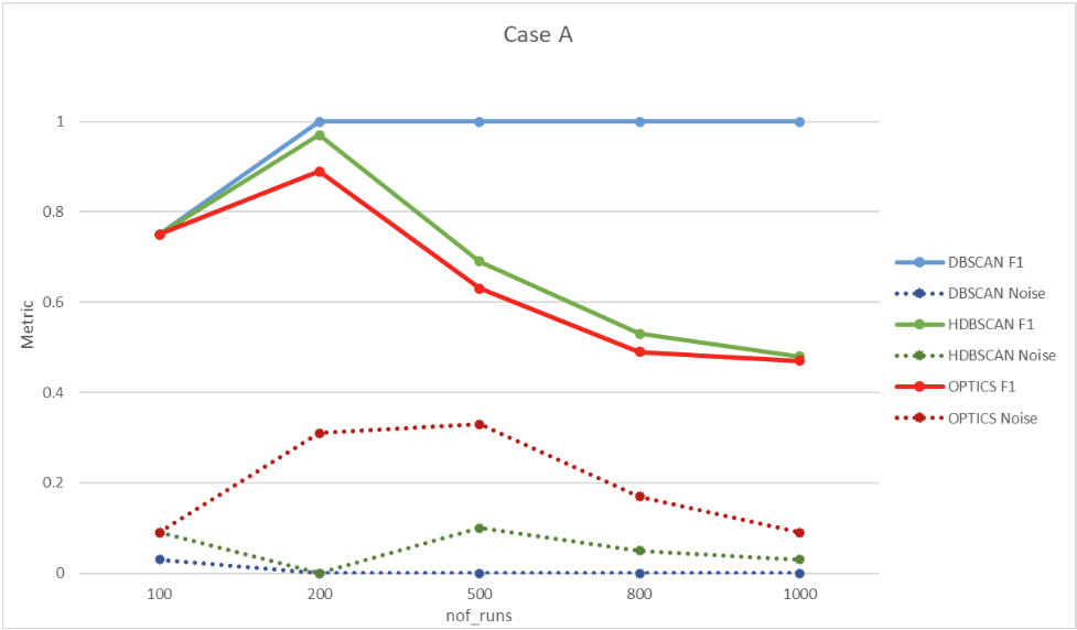
Figure 17. Case A clustering evaluation results.
6.2. Case B – 1:N
In this case, the seed used is 3. Two sequences are used in the configuration presented in the Developer Mode User Guide. Four bugs are generated, one of which is associated with two different error messages. Clustering evaluation results are shown in Figure 18.
| Nof_runs \ Algortihm accuracy | DBSCAN F1 | DBSCAN Noise | HDBSCAN F1 | HDBSCAN Noise | OPTICS F1 | OPTICS Noise |
| 100 | 0.67 | 0.09 | 0.00 | 1.00 | 0.67 | 0.09 |
| 200 | 0.75 | 0.03 | 0.75 | 0.03 | 0.75 | 0.03 |
| 500 | 1.00 | 0.00 | 1.00 | 0.00 | 1.00 | 0.00 |
| 800 | 1.00 | 0.00 | 0.79 | 0.20 | 0.75 | 0.46 |
| 1000 | 1.00 | 0.00 | 0.68 | 0.11 | 0.74 | 0.32 |
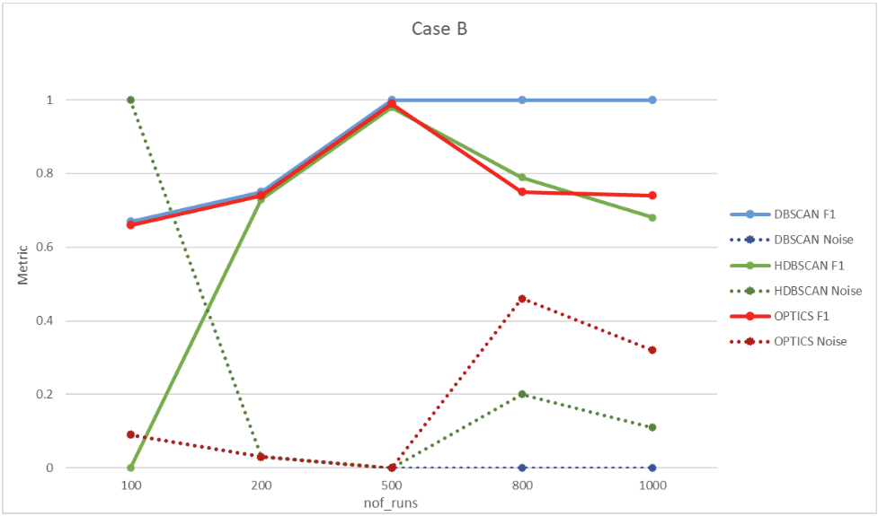
Figure 18. Case B clustering evaluation results.
6.3. Case C – Nested bugs
The seed used is 7. Two sequences are used, in the same configuration as Case B from the previous section. Four bugs are generated, one of which is nested within another bug (one bug involves two values, while the other extends the first values with an additional one). The clustering evaluation results are depicted in Figure 19.
| Nof_runs \ Algortihm accuracy | DBSCAN F1 | DBSCAN Noise | HDBSCAN F1 | HDBSCAN Noise | OPTICS F1 | OPTICS Noise |
| 100 | 0.50 | 0.30 | 0.00 | 1.00 | 0.44 | 0.00 |
| 200 | 1.00 | 0.00 | 0.75 | 0.14 | 1.00 | 0.00 |
| 500 | 1.00 | 0.00 | 0.92 | 0.03 | 0.90 | 0.17 |
| 800 | 1.00 | 0.00 | 0.64 | 0.12 | 0.65 | 0.13 |
| 1000 | 1.00 | 0.00 | 0.52 | 0.11 | 0.47 | 0.27 |
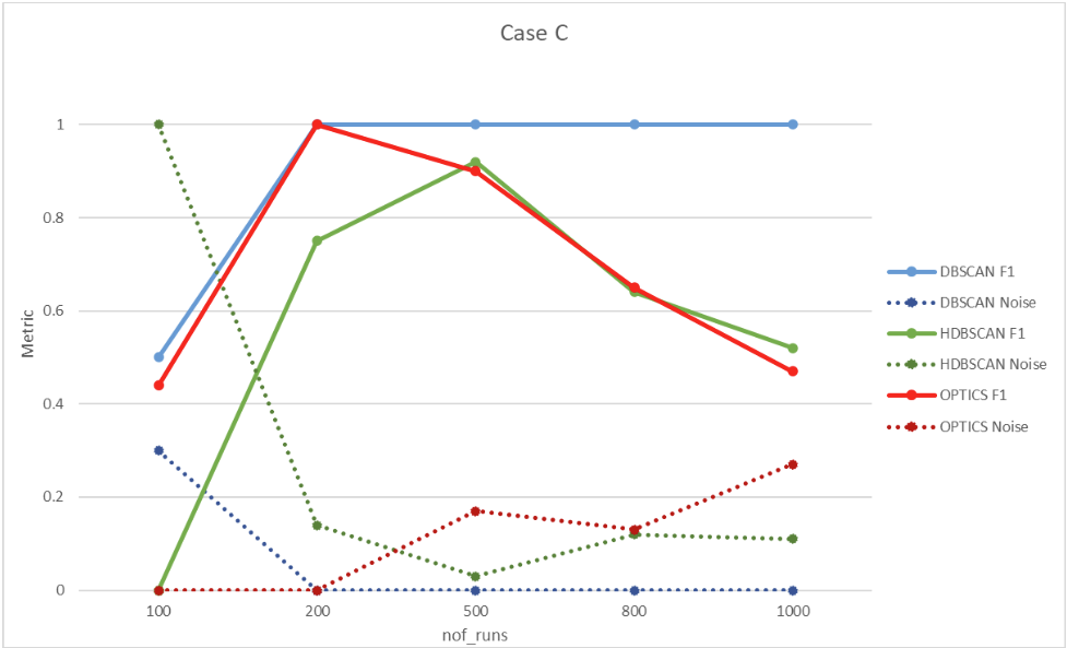
Figure 19. Case C clustering evaluation results.
7. Conclusions
Identifying error root-causes through a graphical application with clustering capabilities is feasible and significantly reduces the debugging time for functional verification engineers. Moreover, it eliminates the need to analyze waveforms and to iteratively investigate simulations. The proposed clustering methodology provided the best results using the DBSCAN algorithm within the sandbox environment, and the project scales with the number of verification environment parameters, the number of sequence types used, the number of existing bugs, as well as with the number of runs in a regression.
The sandbox environment is an adequate solution for developing this project, but the major step that needs to be taken in using this regression failure triage tool is an industry-level project, with real bugs. With provided feedback, it could be determined if this project can be used for accelerating debugging, predicting the number of bugs in an architecture, or better visualizing and understanding regression results.
8. References and resources
- https://blogs.sw.siemens.com/verificationhorizons/2022/12/12/part-8-the-2022-wilson-research-group-functional-verification-study/
- https://www.geeksforgeeks.org/clustering-in-machine-learning/
- https://file.biolab.si/papers/1996-DBSCAN-KDD.pdf
- https://www.khoury.northeastern.edu/home/vip/teach/DMcourse/2_cluster_EM_mixt/notes_slides/revisitofrevisitDBSCAN.pdf
- https://scikit-learn.org/stable/modules/clustering.html#dbscan
- https://link.springer.com/chapter/10.1007/978-3-642-37456-2_14
- https://dl.acm.org/doi/pdf/10.1145/304181.304187
- https://www.consulting.amiq.com/2023/01/30/amiq-ectb-externally-controlled-testbench-architecture-framework/
- https://jmlr.csail.mit.edu/papers/volume12/pedregosa11a/pedregosa11a.pdf
- https://plotly.com/dash/
- https://www.jstor.org/stable/2528823
- https://www.semanticscholar.org/paper/Measures-of-the-Amount-of-Ecologic-Association-Dice/23045299013e8738bc8eff73827ef8de256aef66
- https://plotly.com/python/sankey-diagram/
- https://www.sciencedirect.com/science/article/pii/S0169023X06000218
- https://ieeexplore.ieee.org/document/7035339
- https://www.sciencedirect.com/science/article/pii/0024379585901879?ref=pdf_download&fr=RR-2&rr=8d9648194cd370d1
- https://www.geeksforgeeks.org/categorical-data/
- https://www.geeksforgeeks.org/k-nearest-neighbours/
- https://www.consulting.amiq.com/wp-content/uploads/2025/01/Developer-Mode-User-Guide.pdf
9. Acknowledgements
I want to express my gratitude towards all of my AMIQ colleagues, especially to those directly implicated: Mihai Cristescu for orchestrating, Bogdan Iordache for inspiring, and Andrei Vintila for driving this project forward.